The definition and reduction of the genetic regulatory network under study gives rise to a schema summarizing the relevant genes, proteins, and interactions. In the next step, this schema is transformed into a GNA model of the network, by adding more information on the regulation of the genes. A GNA model has the form of a system of piecewise-linear differential equations (PLDEs), completed by a set of inequality constraints. The formulation of the model will be illustrated here, by means of the simple example introduced in the previous section.
The model-building process consists of four steps:
Definition of state and input variables
Definition of parameters
Definition of state equations
Definition of inequality constraints
The model-building process can be automated to some extent by means of a model-building wizard. Each of the above steps, and their integration with the model-building wizard, is discussed in detail below.
Most of the time, you will not build a model from scratch, but start
from an earlier model. In that case, you choose in the menu to load the
earlier model you have decided to use as a template. You may import models
from earlier GNA versions (text files with the extension .gna) by choosing in the menu. It is also
possible to import a model in SBML format, by choosing in the same menu.
In the case a model does not have an associated network, defined as in
Section 2.1, the Reduced network window is absent.
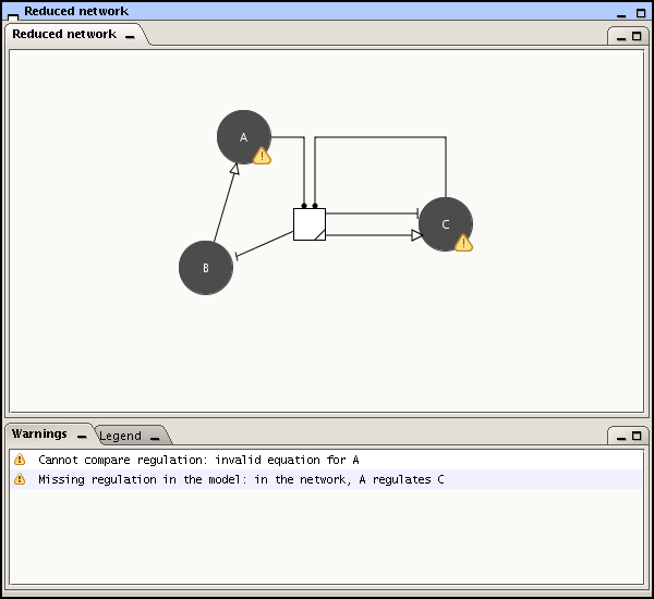
In order to complete the network into a PLDE model, you have to click the tab in the left-upper corner of the application. GNA opens a desktop with two components: the Project tree and the Reduced network window. The project tree lists the variables of the model as well as the initial conditions, atomic propositions and properties, while the Reduced network window shows the network of direct and indirect genetic regulatory interactions as obtained through reduction (see Figure 2.4).
The Reduced network window is also a way to check the consistency of the model definition with the network schema. It will graphically indicate the differences between both representations. The warnings can be ignored and do not impact the modeling, but it is usually advisable to check if the differences are intentional or not. Warnings are produced in the following cases:
A network element does not exist as a model variable;
A variable created in the model has no corresponding element in the network;
The regulation of a variable differs between the network and the model (e.g., in Figure 2.4 the regulation of C by A cannot be found in the state equation for C);
The equation for a state variable is invalid.
The genes in the network correspond to variables in the model,
representing the concentrations of the proteins encoded by the genes.
The variables are created by choosing the option in the menu. You can also
press the button of your mouse when the
cursor is on the model item in the Project window.
In the remainder of this page, we will omit the shorthand commands for
menu options, which are listed in the overview of GNA functions. The
creation of a variable is accomplished by specifying its name and leads
to the opening of the Variable window. In the case
of the example network, three variables are defined:
x_a, x_b, and
x_c. After their creation, variables can be renamed
or deleted, by means of the options and in
the menu.
Two different types of variables are distinguished: state variables and input variables. While the former vary as a function of the other concentration variables in the model, the latter are determined by factors outside the scope of the system. In addition, GNA assumes that they are constant. In the Variable window, a variable can be defined as an input variable. This hides a number of fields in the Variable window that are irrelevant for input variables, or makes them inaccessible.
The Variable window also allows you to
specify a number of parameters. Upon creation of a state or input
variable, a zero parameter and a
maximum parameter are automatically
defined in the parameter tree on the
left. The zero and maximum parameters indicate a lower and upper bound
for the concentration of the protein, respectively. By selecting these
parameters in the parameter tree, the default name assigned by GNA can
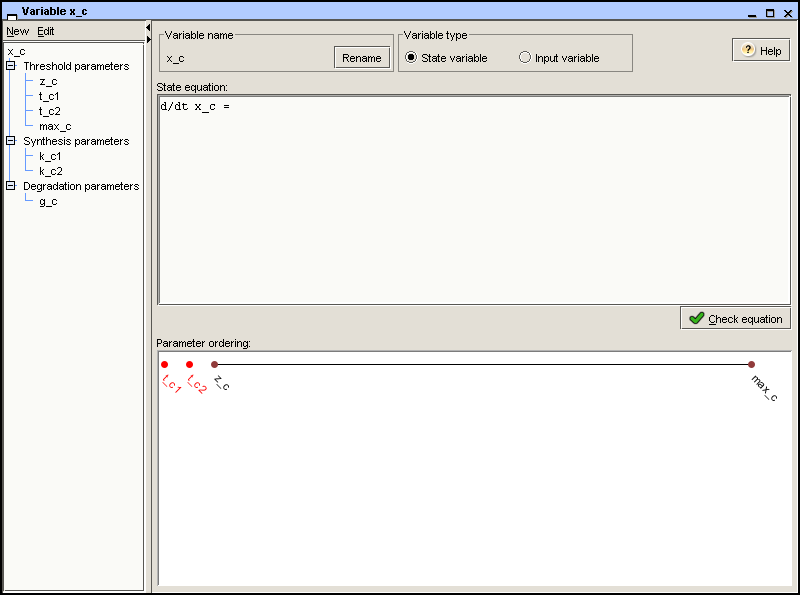
be changed. For the variable x_c, we define a zero
parameter zero_c and a maximum parameter
max_c, as shown in Figure 2.5 below.
The parameter tree may also contain a number of threshold parameters for the variable. A
threshold indicates the concentration above or below which a regulatory
protein has an influence on the expression of the target gene. As a
protein may be involved in several regulatory interactions, it may have
several different thresholds The thresholds are created by pressing the
button of the tree menu, which asks the name
of the threshold and inserts the newly created threshold into the tree.
Once created, a threshold parameter can be deleted or renamed. In the
case of x_c, we define thresholds
t_c1 and t_c2, arising from the
two interactions in which the protein encoded by gene
c is involved. Notice that, if two thresholds are
equal, they are given the same name.
Finally, if the variable is a state variable, you can specify
so-called synthesis and degradation parameters. These indicate the rate
of synthesis and degradation, respectively, of the protein whose
concentration is represented by the variable. The synthesis and
degradation parameters are specified in the parameter tree. The same
buttons and allow
the parameters to be created and maintained. Because there must always
be at least one degradation parameter, GNA creates one by default. In
the example, we introduce two synthesis parameters for
x_c, k_c1 and
k_c2, representing two possible synthesis rates of
protein C, respectively. In addition, we introduce the degradation
parameter g_c. The result is shown in Figure 2.5.
Next, still in the Variable window, we add information on the regulatory logic of the synthesis and the degradation of the proteins. That is, we specify state equations, which define the rate of change of the protein concentrations as a balance between the synthesis and the degradation rates of the protein. The state equations are entered in the State equation field, according to the syntax of GNA models specified in the appendix.
The synthesis term of the state
equation is a sum of step-function
expressions, each weighted by a synthesis parameter. Recall
that, in the case of protein C, we defined two synthesis rates,
k_c1 and k_c2, respectively.
Suppose that the protein is not produced at all, if the concentration of
protein C is above its threshold t_c2. That is, for
x_c > t_c2, negative autoregulation of the gene
sets in. On the other hand, for xc < t_c2, the
protein is produced at a rate which is assumed to depend on the
concentration of protein A. If the latter concentration is below the
threshold t_a2, i.e.
x_a < t_a2, then gene c is
expressed at a low rate k_c1. However, if
x_a > t_a2, then RNA polymerase is stabilized by
protein A, and gene c is expressed at a high rate
k_c1 + k_c2. The following synthesis term captures
this regulatory logic: k_c1 * s-(x_c,t_c2) + k_c2 *
s-(x_c,t_c2) * s+(x_a,t_a2), where
s-(x_c,t_c2) and s+(x_a,t_a2) are
step-function expressions. That is, s-(x_c,t_c2)
evaluates to 1, if x_c < t_c2, whereas it
evaluates to 0, if x_c > t_c2. The case of
s+(x_a,t_a2) goes analogously, while bearing in mind
that s+(x_a,t_a2) = 1 – s-(x_a,t_a2).
The degradation term is defined
analogously to the synthesis term, except that we demand that an
unregulated, spontaneous degradation term is included, in order to
ensure that the degradation rate of the protein is always positive. If
we only have spontaneous degradation or growth dilution, as in the
example of Figure 2.6, then the
degradation term is simply a degradation parameter multiplied by the
state variable (e.g., g_c *
x_c). In case the degradation of the protein is also regulated
by other proteins, one or more step-function expressions, each weighted
by a degradation parameter, are added to the degradation parameter
accounting for spontaneous degradation. The resulting sum is multiplied
by the state variable. For example, above a threshold concentration
t_b2, protein B might favor degradation of protein C,
by binding to it and thus presenting it to the proteolytic machinery.
This can be represented by the degradation term (g_c1 + g_c2 *
s+(x_b,t_b2)) * x_c, where g_c1 is a low,
spontaneous degradation rate, and g_c1 + g_c2 a high,
regulated degradation rate.
In general, the step-function expressions in the synthesis and the degradation terms may take many forms, depending on the number of proteins involved and the regulatory logic they implement. Further examples of step-function expressions, sometimes quite complex, can be found in the model of the initiation of sporulation in B. subtilis and the model of the carbon starvation response in E. coli.
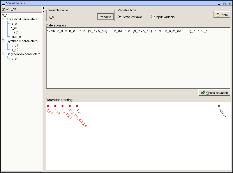
The state equation is a differential equation whose righthand-side
is the difference of the synthesis and degradation terms. In the
example, the state equation for protein C is d/dt x_c = k_c1 *
s-(x_c,t_c2) + k_c2 * s-(x_c,t_c2) * s+(x_a,t_a2) – g_c * x_c,
as shown in Figure 2.6. Once entered
in the State equation field, the syntax and
semantics of the state equation can be checked by clicking the
button. It is then verified that
the equation satisfies the syntax of GNA
models and that it is consistent with the parameter definitions
in the other Variable windows.
The simulation method does not require precise numerical values for the threshold, synthesis, and degradation parameters. Instead, inequality constraints on the parameter values are specified to predict the qualitative dynamics of the regulatory system (see the section on running simulations). More precisely, GNA demands the user to order the so-called threshold parameters and focal parameters. We briefly explain the biological meaning of these parameters and their ordering by means of the example.
Protein C has two thresholds, t_c1 and
t_c2. Assume that the protein influences the
expression of gene b at lower concentrations than
it influences the expression of its own gene. This gives rise to the
inequality t_c1 < t_c2. By default,
zero_c < t_c1 and t_c2 <
max_c. The thresholds divide the phase space into regions in
which the step functions evaluate to either 0 or 1, so that the state
equations there reduce to linear and uncoupled differential equations.
Inside a region, each protein concentration monotonically converges
towards a so-called focal parameter,
given by a quotient of synthesis and degradation parameters of the
protein. The state equation above, for instance, implies that in a
region in which x_a lies below
t_a2, and x_c below
t_c2, x_c converges towards the
focal parameter k_c2/g_c. The behavior of the system
on the threshold planes separating the regions can be determined from
the behavior in the adjacent regions, as explained in the publications on the
qualitative simulation method.
The possible focal parameters in the different regions of the
phase space can be ordered with respect to the threshold parameters.
Intuitively speaking, this defines the strength of gene expression in
the regions of the phase space in a qualitative way, on the scale of
ordered threshold concentrations. In the case of variable
x_c, the possible focal parameters are 0,
k_c1/g_c, and (k_c1 + k_c2)/g_c.
At the highest expression level, corresponding to the focal parameter
(k_c1 + k_c2)/g_c, protein C should be able to
repress its own synthesis. This implies that t_c2 < (k_c1 +
k_c2)/g_c < max_c. In addition, we set t_c1 <
k_c1/g_c < t_c2.
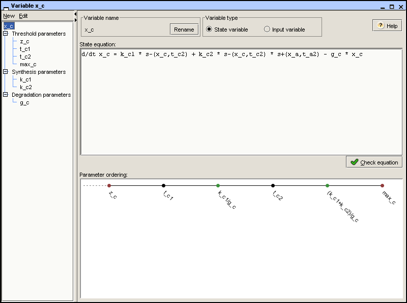
The ordering of the threshold and focal parameters, and thus the
specification of the inequality constraints, is achieved in the
Parameter ordering field. It contains an axis on
which the previously defined threshold, zero, and maximum parameters, as
well as the focal parameters automatically generated from the state
equation are positioned. The elements of the list can be ordered by
means of the mouse, by dragging them up and down the axis. Elements can
also be moved out of the ordered list, by dropping them left from the
zero parameter. Notice that this results in a total order of the
threshold and focal parameters, contrary to what was the case in
previous versions of GNA (in which focal parameters did not need to be
totally ordered with respect to each order). As a consequence, when
models prepared with previous versions of GNA (version 6.0 or below) are
loaded in GNA 8, the program issues a warning that the parameter order
is not total and appends the unordered focal parameters at the left of
the zero parameter. Figure 2.7
shows the ordered threshold and focal parameters for the variable
x_c.
After you have specified the inequality constraints, the GNA model
of the genetic regulatory network is complete. You can save it by means
of or in the menu. The project is
saved in an XML file with the extension .xml or .gnaml. You may also decide to export the
model to a file with the .gna
extension (former GNA files) by the means of in the menu, or even
export it to SBML using .
Examples of complete model files can be consulted in the samples directory of the GNA
distribution.
The first three steps of building a model (definition of state and input variables, definition of parameters and definition of state equations) can also be handled through a wizard that allows you to semi-automatically complete these steps. The model definition wizard is available if you have previously defined a network. It is launched the first time you switch from the network to the model editor mode. Even if the wizard is capable of dealing with only a resttricted range of regulating mechanisms and may thus not give correct results for complex networks, it is usually worth the effort to run it in order to prepare a basic - perhaps partial - model that will facilitate and speed up the rest of the modeling process.
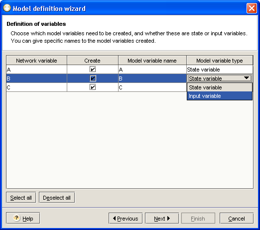
The first step of the wizard allows you to decide which variables will be created in the model (see Figure 2.8). The default proposal is based on the following rules:
Genes and external signals will be used to create corresponding model variables;
Among these variables, those regulated by other variables will be tagged as state variables;
Other variables, not regulated, will be tagged as input variables and will not have a state equation associated. This will allways be the case for external signals.
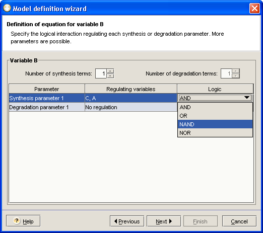
The second step of the wizard consists in defining an equation for each state variable you want to take into account (you may decide not to let the wizard algorithm generate some of the equations and define them by yourself later on). For a specific state variable, the wizard takes all regulating variables into account and uses AND logic to generate a consistent equation. You can specify various parameters, such as the number of synthesis and degradation parameters, the variables implied for each of these parameters, and the regulatory logic applied (you can choose between AND, NAND, OR and NOR). This is illustrated in Figure 2.9. When the options fit your needs, click on the button to reach the next step of the wizard.
When working with the wizard, you can go back one or more steps, or even cancel the process. When you have successfully completed all steps of the wizard, you still have to order the parameters for each variable. After this you can start specifying initial conditions and further simulating and analyzing the model.