The Results page in the Simulation window summarizes the results obtained for a qualitative simulation (Figure 2.12). It displays the qualitative steady states and qualitative cycles that are reachable from the initial qualitative states, as well as the attraction set of each qualitative steady state or qualitative cycle (i.e., the set of qualitative state from which the attractor is reachable). The Results page in the Simulation window also gives the name of the Transition graph window, containing the state transition graph resulting from the simulation (Figure 2.13). In the example, the state transition graph consists of 50 qualitative states, associated with domains lying between threshold or focal planes (regulatory domains), or domains lying on one or more threshold or focal planes (switching domains). In order to graphically distinguish the qualitative states associated with regulatory and switching domains, the former have an emphasized border. In addition, to facilitate visual inspection of the graph, qualitative steady states are shaded.
Fig. 2.12. Simulation window displaying results of a qualitative simulation of the genetic regulatory network in Figure 2.1: Qualitative steady states, qualitative cycles, and their attraction sets
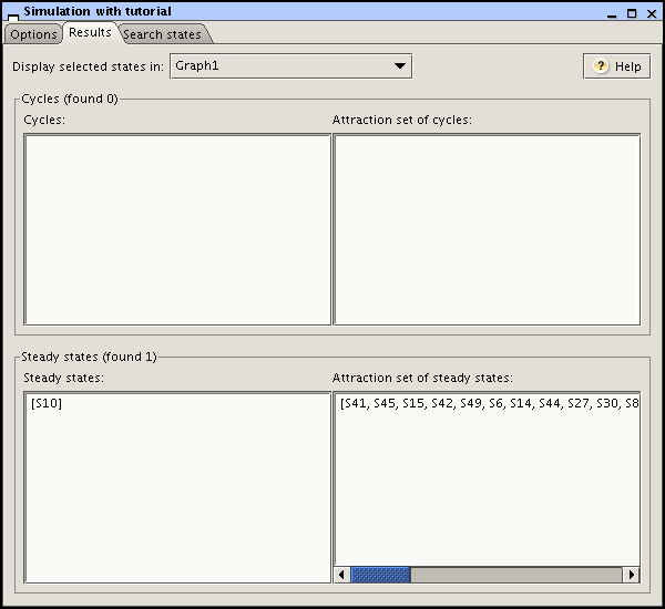
Fig. 2.13. Results of a qualitative simulation of the genetic regulatory network in Figure 2.1: Fragment of the state transition graph
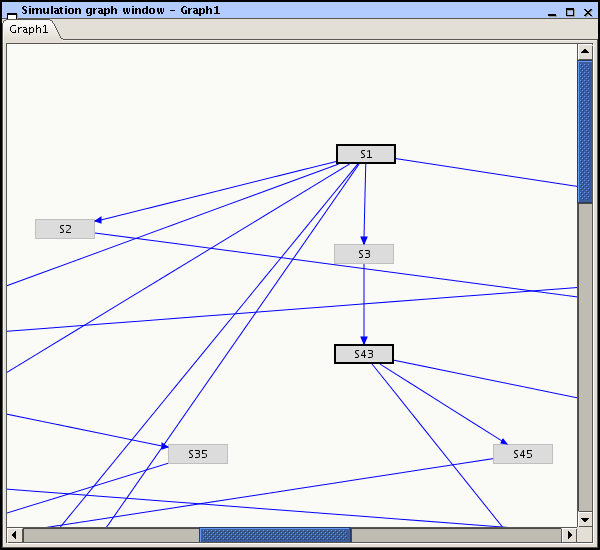
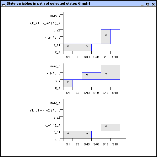
The state transition graph contains more detailed information on the qualitative dynamics of the system, which can be analyzed by means of the graphical user interface. First, by hovering the mouse cursor on a qualitative state, the properties characterizing the state, notably its location in the phase space, are displayed in textual form. Press the F2 key if you want to focus on it. Second, you can select a path in the state transition graph and use the option in the menu to show the qualitative evolution of the protein concentrations along the selected path. The states are selected by means of the mouse, while pressing the Ctrl key. A click on a selected state, again while pressing the Ctrl key, allows this state to be deselected. In Figure 2.14, you can see a path selected in the state transition graph of Figure 2.13. Notice that the order in which the states have been selected determines the order in the concentration profiles shown. If the selected order is consistent with the successor relations in the state transition graph, then the path can be interpreted as a temporal order of events. More precisely, the concentration profile then shows how the derivative signs of the variables evolve over time, giving rise to a sequence of maxima and minima for each of the variables. This information can be straightforwardly compared with available gene expression data. Similarly, the option in the menu shows the qualitative evolution of the values towards which the state variables locally converge.
Fig. 2.14. Qualitative evolution of the variables
x_a, x_b, and
x_c in a path selected in the state transition graph
of Figure 2.13
For more complex genetic regulatory networks, the state transition graph produced by GNA may contain hundreds or thousands of states. Depending on the display limit set in the Properties page of the Simulation window, only part of the state transition graph is then displayed. The graphical user interface provides a few functions to analyze this graph. First, the zoom functions in the menu - more conveniently accessed through the mouse button (see the overview of GNA functions) - allow you to increase or decrease the visible part of the graph. Second, you can select a subset of the state transition graph, display it in a separate tab, and expand it using several levels of successors and/or predecessors. Third, a useful option is to reduce the graph by eliminating qualitative states that correspond to domains that are instantaneously traversed, and therefore have no practical relevance. This option, called in the menu, eliminates 32 of the 50 qualitative states of the state transition graph in our example. Fourth, the Search states page in the Simulation window allows you to identify parts of the state transition graph that satisfy certain search criteria. Finally, once a single state is selected it is possible to navigate through the transition graph using the keyboard arrows (maintain the Alt key pressed to add new states to the selection).
For really large models, the above functions may not be sufficient, and other solutions need to be tried. GNA offers two functionalities that are of particular interest for the analysis of large state transition graphs. First, you can export your graph to a model-checking tool and further analyze its properties by formulating queries in a temporal logic (see section on checking properties of the state transition graph). Second, instead of generating the entire state transition graph, you can use the attractor search option (see the section on searching for attractors).