Another way to deal with large state transition graphs is to analyze
the graph by means of formal verification techniques, implemented in
computer tools called model checkers. Examples of the kind of properties
one might want to test are "It is possible for a state with an
x_a concentration equal to t_xa2 to
occur" or "If the system is in the state
corresponding to the initial conditions zero_a <= x_a <
t_a1, zero_b <= x_b < t_b, and
zero_c <= x_c < t_c1, then it necessarily reaches
a steady state".
The use of the model-checking tools involves three steps:
The specification of the property to be verified by defining atomic propositions and formulating so-called temporal-logic formulas;
The actual verification of the property by a model checker.
An atomic proposition is used to characterize qualitative states. It indicates, for each variable in the model, its value, the value toward which it converges, the sign of its derivative. In addition, it specifies state descriptors indicating, e.g., whether the state is a steady state.
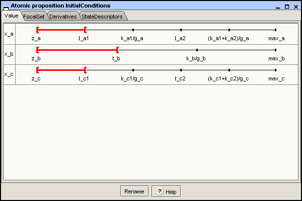
An atomic proposition can be created by means of in the Edit menu: a new atomic proposition is created and the corresponding Atomic proposition window opens (see Figure 2.16). The window is composed of 4 tabs:
the Value tab, where the user can choose (strict) lower and upper bounds for the value of each variable (following the same principle as the specification of the initial conditions);
the FocalSet tab, where the user can choose (strict) lower and upper bounds for the focal value of each variable. Within each region of the state space, the system converges towards a so-called focal set (see the publications on GNA);
the Derivatives tab, where for each variable, the user can select the appropriate derivative sign (Undefined, Zero, Positive, Negative, All);
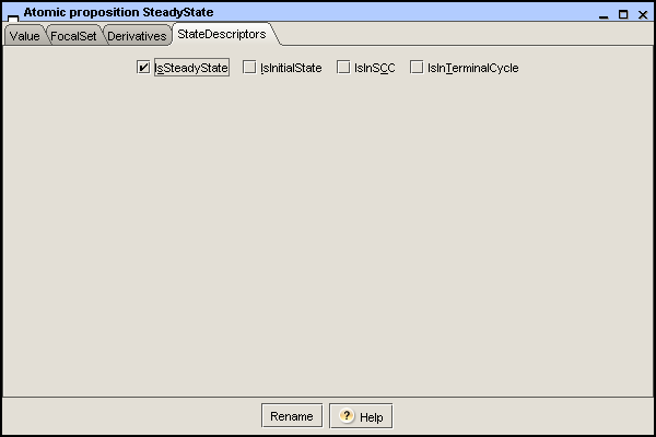
the StateDescriptors tab contains check boxes that can be selected if the user wants to specify that the state is a steady state, an initial state, in a strongly connected component, or in a terminal cycle of the state transition graph.
A newly created atomic proposition has a default specification, which does not impose any specific constraints and is thus true for all states in the state transition graph.
In order to verify the property "If the system is in the
state corresponding to the initial conditions zero_a <= x_a
< t_a1, zero_b <= x_b < t_b, and
zero_c <= x_c < t_c1, then it necessarily
reaches a steady state", we need to create two atomic
propositions. One is called InitialConditions and
specifies the initial conditions zero_a <= x_a <
t_a1, zero_b <= x_b < t_b, and
zero_c <= x_c < t_c1. The other is called
SteadyState and specifies that the state is a steady
state (see Figure 2.16).
Fig. 2.16. Atomic proposition windows, showing the
specification of the atomic propositions
InitialConditions and
SteadyState.
The atomic propositions are included in the temporal-logic property, defined by means of a special editor. The use can call the editor by opening the menu and choosing the item. It opens the Property editor window which is composed of two tabs, corresponding to two different ways to formulate a property. The first is a pattern-based wizard that allows you to formulate a property without any knowledge of temporal logic. The second is a free-text interface that provides all the flexibility of the temporal logic supported by GNA, called CTRL. This logic subsumes standard temporal logics like CTL and LTL (see GNA publications).
A pattern is a high-level query template that captures recurring questions and can be automatically translated into temporal logic.
Four different patterns, each with some variants, are available to the user. Together they cover most of the frequently-asked questions by modelers (see GNA publications).
Occurrence: It is (not) possible for a state satisfying an atomic proposition
pto occur;Consequence: If a state satisfying an atomic proposition
poccurs, then it is possibly (or necessarily) followed by a state satisfying an atomic propositionq;Sequence: A state statisfying an atomic proposition
qis reachable and is possibly (or necessarily) preceded at some time (or all of the time) by a statep;Invariance: A state satisfying an atomic proposition
pcan (or must) persist indefinitely.
In the pattern wizard, you first click on the radio button for the pattern of your choice, and then use the combo boxes to choose existing atomic propositions and the specific pattern variant of interest (the default choice for the atomic propositions is true).
Once the pattern has been completely specified, you need to click
on the Use selected Pattern button to make the
temporal logic translation of the property appear in the text area at
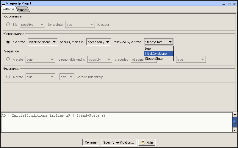
the bottom of the window. This is illustrated by Figure 2.17 for the property
"If the system is in the state corresponding to the initial
conditions zero_a <= x_a < t_a1,
zero_b <= x_b < t_b, and zero_c <=
x_c < t_c1, then it necessarily reaches a steady
state". The property is defined as a Consequence pattern, using the previously-defined
atomic propositions InitialConditions and
SteadyState.
Fig. 2.17. Pattern wizard of the property editor,
showing the pattern definition of the property "If the
system is in the state corresponding to the initial conditions
zero_a <= x_a <
    t_a1
, zero_b <=
x_b < t_b, and zero_c <= x_c <
t_c1, then it necessarily reaches a steady state"
and its translation into temporal logic.
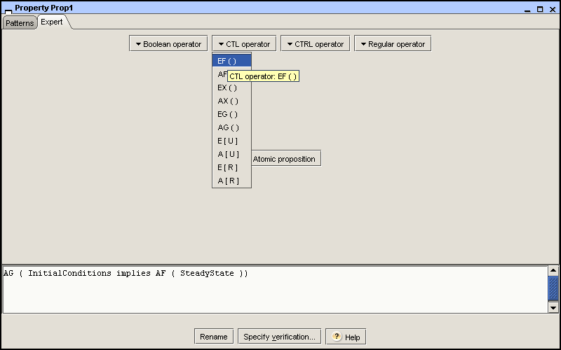
If you are comfortable with the CTRL temporal logic, you can alternatively select the Expert tab. This allows you to directly enter the property by typing it in the text area. Another way to edit a property is by using the combo box system, selecting the corresponding operators and atomic propositions, which are directly inserted in the text area, as shown in Figure 2.18. To check if the temporal logic specification of the property is well-formed and compliant with the CTRL grammar, you can choose the Check syntax button.
The temporal-logic properties and atomic propositions are saved in
the same project file of the model. However, they can also be imported
and exported as files with the extension .prop (see the appendix on the syntax of CTRL
properties for details). To this end, use the
and
items in the menu.
Fig. 2.18. Expert tab of the property editor, used for specifying the same property as in Figure 2.17
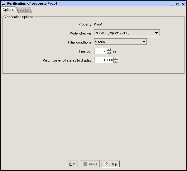
Once the temporal logic formula has been completely specified, you can check its validity by means of the model-checking server in two different ways: either through the property editor, by clicking on the button, or through the item with the same name in the Analysis menu. In both cases, a Verification window is opened for the property to be verified. An example is shown in Figure 2.19.
The Verification window asks you to specify the options of the model-checking process. The first option concerns the model checker. The choice of a model checker is constrained by the temporal logic used to specify the property and the available plugins. By default, the GNA distribution includes plugins for the NuSMV model-checker, which makes GNA capable of verifying properties specified in CTL. Plugins for other model-checkers are available on the GNA website.
After choosing a model checker, the corresponding graph type is automatically selected. To each of the registered model checker is associated one of the following graph types:
The explicit graph is an explicit export of the state transition graph previously obtained by running a simulation for a given set of initial conditions. If the graph is too big, it is not possible to use the model-checker web server;
The implicit graph is a model-checker specific model description, containing all the necessary rules for the generation of the successors states by the model checker. This avoids having to run a simulation in GNA and ensures that a smaller file is sent through the web-server connection.
If the explicit graph is selected, you must choose one of the previously simulated state transition graphs. If the implicit graph is selected, you must choose one of the previously defined initial conditions.
When clicking on the Run button, a verification request consisting of an (implicit or explicit) graph and a temporal-logic property is sent to the model-checker server. At any time you can abort the verification by clicking on the Abort button.
Once the verification is completed, a result is returned by the model-checker server. This consists of two elements, displayed in the Results tab of the frame:
a verdict (true/false/error), representing the result of the property verification;
a diagnostic graph, containing an example or a counterexample (if one exists). In the explicit case, this counterexample will be a subgraph of the state transition graph sent to the model checker.
If the verdict is true, the diagnostic graph represents a path that shows the property to be correct. On the contrary, if the verdict is false, the diagnostic graph represents a path that contradicts the property.
Fig. 2.19. Verification window. Specification of the model checker options for the verification of the property defined in Figure 2.17
In case you do not wish to use the model-checker server, or if the
model-checker server is not available, you can also directly test your
property in the model checker of your choice. To this end, install the
model checker locally on your computer and export the (explicit or
implicit) graph in the appropriate format. With the default plugins in
the GNA distribution, the menu has an
item that allows you to generate files
that can be read by NuSMV (.smv).
You can also generate the graph from the console using the command
explained in Section 2.4. The supported
formats are determined by the available plugins.
Examples of properties to be tested for several models in the GNA
distribution can be consulted in the samples directory.

